ディープラーニングのロジスティクス回帰をPythonで実装した例をご紹介

ロジスティック回帰を実装する際のポイント（実装のステップ）と、Pythonで実装したサンプルコードをご紹介します。

※ロジスティック回帰とは？について知りたい方はこちらもご覧ください。

⇒（参考）ロジスティック回帰とは？Excelで計算する方法もご紹介（★）

・入力の電気信号xの初期化

・重みwの定義

・バイアスbの定義

・出力層（シグモイド関数）：y = σ(wx + b)の定義

・正解値tの定義

・重みwの勾配（∂E(w,b)/∂w）の定義

・バイアスbの勾配（∂E(w,b)/∂b）の定義

・学習率：ηの定義

↓

・交差エントロピー誤差関数：E(w,b) = -Σ[n=1…N]{tn*log(yn) + (1-tn)*log(1-yn)}

⇒今回は不要（確率的勾配降下法を使うため、誤差関数Eは計算不要）

↓

・シグモイド関数：y = σ(wx + b)の計算

・重みwの勾配（∂E(w,b)/∂w）の計算

・バイアスbの勾配（∂E(w,b)/∂b）の計算

・重みwの再計算

・バイアスbの再計算

↓

⇒今回は不要（TensorFlow v2以降はSessionを使用しないため）

↓

・ループ変数の範囲で処理を繰り返す。

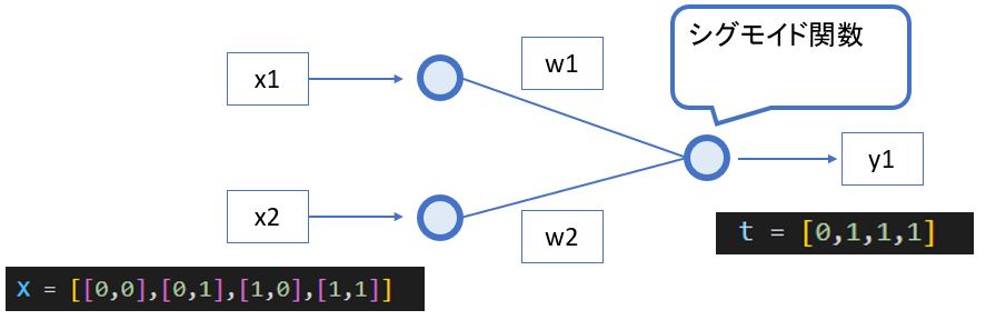
今回はOR回路を学習させた例をご紹介します。

（図１２０）

（サンプルプログラム）

import numpy as np
import tensorflow as tf
import os
os.environ['TF_CPP_MIN_LOG_LEVEL'] = '3'

# 入力xの次元
M = 2
# 入力データセットの数
N = 4
# ミニバッチの数
#n_batch = 4

def or_gate(X_arg,t_arg):
    ############################################
    # STEP1：モデルの定義
    ############################################
    # 入力の電気信号xの初期化
    X = tf.constant(X_arg, dtype = tf.float64, shape=[N,M])
    # 重みwの定義　⇒[1行×M列]
    weight = tf.Variable(tf.zeros([M],tf.float64), dtype = tf.float64, shape=[M])
    # バイアスbの定義　⇒[1行]　
    bias = tf.Variable([0], dtype = tf.float64, shape=[1])
    # シグモイド関数：y = σ(wx + b)の定義　⇒[1行]
    y = tf.Variable([0], dtype = tf.float64, shape=[1])    
    # 正解値tの定義（[[0,1,1,1]）　⇒[n行×1列]
    t = tf.Variable(t_arg, dtype = tf.float64, shape=[N])
    # 重みwの勾配（∂E(w,b)/∂w）の定義
    dweight = tf.Variable(tf.zeros([M],tf.float64), dtype = tf.float64, shape=[M])
    # バイアスbの勾配（∂E(w,b)/∂b）の定義
    dbias = tf.Variable([0], dtype = tf.float64, shape=[1])
    # 学習率ηの定義
    eta = 0.1
    # Epocの定義
    epoc = 0

    ############################################
    # STEP4：セッションの初期化
    ############################################
    # ⇒今回は不要
    # （TensorFlow v2以降はSessionを使用しないため）

    ############################################
    # STEP5：学習
    ############################################
    for epoc in range(25):
        # バッチのデータ数だけ繰り返し
        for n in range(N):
            xn = X[n]
            ############################################
            # STEP2：誤差関数の定義
            ############################################
            # ⇒今回は不要
            # （確率的勾配降下法を使うため、誤差関数Eは計算不要）

            ############################################
            # STEP3：最適化手法の定義（例：勾配降下法）
            ############################################
            # yの計算（モデルの出力）
            # matmul(weight(1×M),X(1×M))
            y = tf.nn.sigmoid(np.dot(xn,weight)+bias)

            # 重みwの勾配（∂E(w,b)/∂w）の計算
            dweight = tf.math.scalar_mul((t[n]-y[0]),xn)
            # バイアスbの勾配（∂E(w,b)/∂b）の計算
            dbias.assign([t[n]-y[0]])

            # 重みwの再計算        
            weight.assign_add(dweight)
            # バイアスbの再計算
            bias.assign_add(dbias)

            # コンソール出力
            decimals = 4
            print("Epoc= ",epoc,
                    "No. = ",   n,
                    "x1,x2 =",  X[n].numpy(),
                    "t =",      '{:01}'.format(tf.convert_to_tensor(t[n]).numpy()),
                    "w1,w2 =",  np.round(weight.numpy(),decimals),
                    "theta =",  np.round(bias.numpy(),decimals),
                    "y =",      '{:06.4f}'.format(tf.convert_to_tensor(y[0]).numpy()),
                    "dw1,dw2 =",np.round(dweight.numpy(),decimals),
                    "db =",     np.round(dbias.numpy(),decimals))

def main():
    # 初期値を設定し学習実行
    X = [[0,0],[0,1],[1,0],[1,1]]
    t = [0,1,1,1]
    or_gate(X,t)

if __name__ == "__main__":
    main()

 

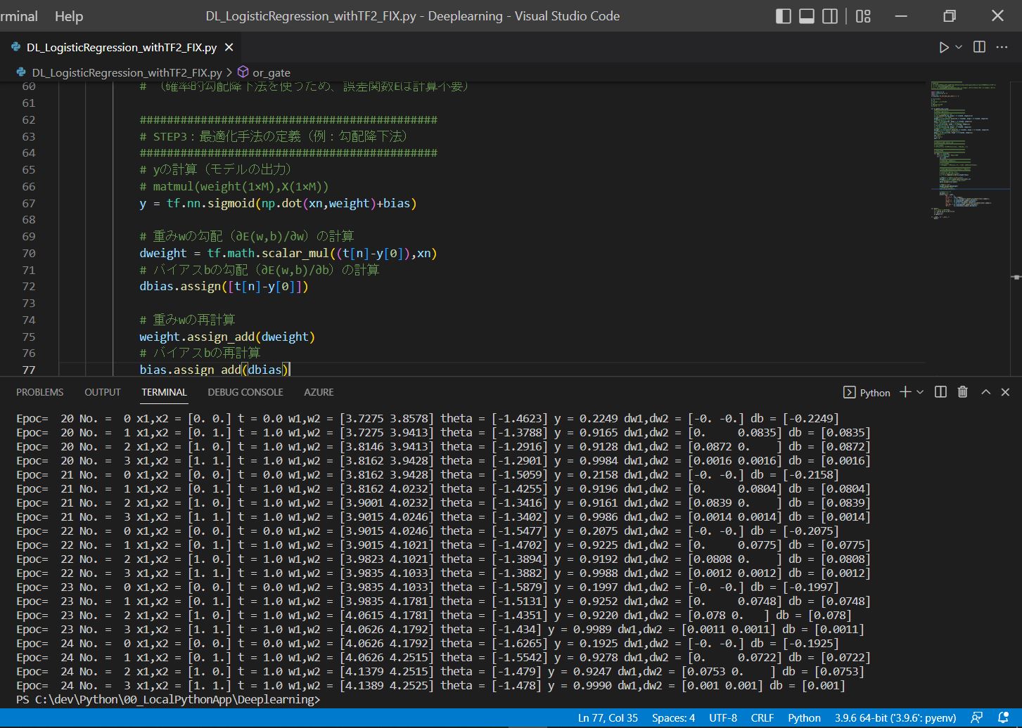
（実行結果）

Epoc=  0 No. =  0 x1,x2 = [0. 0.] t = 0.0 w1,w2 = [0. 0.] theta = [-0.5] y = 0.5000 dw1,dw2 = [-0. -0.] db = [-0.5]
Epoc=  0 No. =  1 x1,x2 = [0. 1.] t = 1.0 w1,w2 = [0.     0.6225] theta = [0.1225] y = 0.3775 dw1,dw2 = [0.     0.6225] db = [0.6225]
Epoc=  0 No. =  2 x1,x2 = [1. 0.] t = 1.0 w1,w2 = [0.4694 0.6225] theta = [0.5919] y = 0.5306 dw1,dw2 = [0.4694 0.    ] db = [0.4694]
Epoc=  0 No. =  3 x1,x2 = [1. 1.] t = 1.0 w1,w2 = [0.626  0.7791] theta = [0.7485] y = 0.8434 dw1,dw2 = [0.1566 0.1566] db = [0.1566]
～中略～
Epoc=  24 No. =  0 x1,x2 = [0. 0.] t = 0.0 w1,w2 = [4.0626 4.1792] theta = [-1.6265] y = 0.1925 dw1,dw2 = [-0. -0.] db = [-0.1925]
Epoc=  24 No. =  1 x1,x2 = [0. 1.] t = 1.0 w1,w2 = [4.0626 4.2515] theta = [-1.5542] y = 0.9278 dw1,dw2 = [0.     0.0722] db = [0.0722]        
Epoc=  24 No. =  2 x1,x2 = [1. 0.] t = 1.0 w1,w2 = [4.1379 4.2515] theta = [-1.479] y = 0.9247 dw1,dw2 = [0.0753 0.    ] db = [0.0753]       
Epoc=  24 No. =  3 x1,x2 = [1. 1.] t = 1.0 w1,w2 = [4.1389 4.2525] theta = [-1.478] y = 0.9990 dw1,dw2 = [0.001 0.001] db = [0.001]

（図１２１）

＞目次にもどる