<目次>
Pythonで多クラスのロジスティック回帰を実装した例をご紹介
実装のフロー
STEP1:モデルの定義
STEP2:誤差関数の定義
STEP3:最適化手法の定義(例:勾配降下法)
STEP4:セッションの初期化
STEP5:学習
サンプルプログラム
Pythonで多クラスのロジスティック回帰を実装した例をご紹介
多クラス分類のロジスティック回帰について、Pythonで実装したサンプルプログラムをご紹介します。
多クラス分類のロジスティクス回帰を実装する際のポイント(実装のステップ)と、Pythonで実装したサンプルコードをご紹介します。
※多クラス分類のロジスティクス回帰とは?について知りたい方はこちらもご覧ください。
実装のフロー
STEP1:モデルの定義
・入力の電気信号xの初期化
・重みWの定義
・バイアスbの定義
・出力層(ソフトマックス関数):y = softmax(Wx + b)の定義
・正解値tの定義
・重みWの勾配(∂E(W,b)/∂w)の定義
・バイアスbの勾配(∂E(W,b)/∂b)の定義
・学習率:ηの定義
↓
STEP2:誤差関数の定義
・交差エントロピー誤差関数:E(W,b) = -Σ[n=1…N]Σ[k=1…K]{t_nk*log(y_nk)}
⇒今回は不要(確率的勾配降下法の最終式を使うため、誤差関数Eは計算不要)
↓
STEP3:最適化手法の定義(例:勾配降下法)
・ソフトマックス関数:y = softmax(Wx + b)の計算
・重みWの勾配(∂E(W,b)/∂W)の計算
・バイアスbの勾配(∂E(W,b)/∂b)の計算
・重みWの再計算
・バイアスbの再計算
↓
STEP4:セッションの初期化
⇒今回は不要(TensorFlow v2以降はSessionを使用しないため)
↓
STEP5:学習
・ループ変数の範囲で処理を繰り返す。
サンプルプログラム
(サンプルプログラム)
import numpy as np
import tensorflow as tf
import os
os.environ['TF_CPP_MIN_LOG_LEVEL'] = '3'
from sklearn.utils import shuffle
import matplotlib.pyplot as plt
# 入力xの次元
M = 2
# 出力yの次元(クラス数)
K = 3
# 入力データセットの総
nc = 10
# 入力データセットの総数
N = nc * K
def mc_logistic_regression(X_arg,t_arg):
############################################
# STEP1:モデルの定義
############################################
# 入力の電気信号Xの初期化
X = tf.constant(X_arg, dtype = tf.float64, shape=[N,M])
xn = tf.Variable(tf.zeros([M,1],tf.float64),dtype = tf.float64, shape=[M,1])
# 重みWの定義
Weight = tf.Variable(tf.zeros([K,M],tf.float64), dtype = tf.float64, shape=[K,M])
# バイアスbの定義 (※データはn個でも1つのbを更新)
bias = tf.Variable(tf.zeros([K,1],tf.float64), dtype = tf.float64, shape=[K,1])
# ソフトマックス関数:y = softmax(Wx + b)の定義 (※データはn個でも1つのyを更新)
y = tf.Variable(tf.zeros([K,1],tf.float64), dtype = tf.float64, shape=[K,1])
# 正解値tの定義
t = tf.Variable(t_arg, dtype = tf.float64, shape=[N,K])
# 重みWの勾配(∂E(W,b)/∂W)の定義
dWeight = tf.Variable(tf.zeros([K,M],tf.float64), dtype = tf.float64, shape=[K,M])
# バイアスbの勾配(∂E(W,b)/∂b)の定義
dbias = tf.Variable(tf.zeros([K,1],tf.float64), dtype = tf.float64, shape=[K,1])
# 学習率ηの定義
eta = 0.1
# Epoc数の定義
epocs = 1000
############################################
# STEP4:セッションの初期化
############################################
# ⇒今回は不要
# (TensorFlow v2以降はSessionを使用しないため)
############################################
# STEP5:学習
############################################
for epoc in range(epocs):
# バッチのデータ数だけ繰り返し
for n in range(N):
# データをシャッフル
X_,t_ = shuffle(X.numpy(),t.numpy())
#X_,t_ = X.numpy(),t.numpy()
# 取り出したX_[n]を転置してxnに格納(Mx1)
xn.assign(tf.transpose([X_[n]]))
############################################
# STEP2:誤差関数の定義
############################################
# ⇒今回は不要
# (確率的勾配降下法を使うため、誤差関数Eは計算不要)
############################################
# STEP3:最適化手法の定義(例:勾配降下法)
############################################
# ソフトマックス関数:y = softmax(Wx + b)の計算
# y[K,1] = softmax( Weight[K×M] × X[M×1] + bias[K×1] )
# reshapeに関しては、softmax関数の引数が[K]の形式でないと適切に動かない為に使用している。
# reshapeで[K]に変換してsoftmaxしたのち、再度[K,1]に戻して行列計算できる形に戻す。
y.assign( tf.reshape( tf.nn.softmax(tf.reshape(tf.matmul(Weight,xn)+bias,[K])),[K,1]).numpy() )
# 重みwの勾配(∂E(W,b)/∂W)の計算
# dWeight[K,M] += ( tn[K×1](転置) - y[K×1] ) × xn[1×M](転置)
dWeight.assign(tf.matmul((tf.transpose([t_[n]])-y),tf.transpose(xn)).numpy())
# バイアスbの勾配(∂E(w,b)/∂b)の計算
dbias.assign( tf.transpose([t_[n]])-y)
# コンソール出力
decimals = 4
print("Epoc= ", epoc+1,
"No. = ", n,
"\r\n\t x1,x2 \t\t=", np.array_repr(np.round(X[n].numpy(),decimals)),
"\r\n\t t \t\t=", np.array_repr(np.round(t[n].numpy(),decimals)),
"\r\n\t w1,w2 \t\t=", np.array_repr(np.round(Weight.numpy(),decimals)).replace('\n', '').replace(' ', ''),
"\r\n\t b \t\t=", np.array_repr(np.round(bias.numpy(),decimals)).replace('\n', '').replace(' ', ''),
"\r\n\t y \t\t=", np.array_repr(np.round(y.numpy(),decimals)).replace('\n', '').replace(' ', ''),
"\r\n\t dw1,dw2 \t=", np.array_repr(np.round(dWeight.numpy(),decimals)).replace('\n', '').replace(' ', ''),
"\r\n\t db \t\t=", np.array_repr(np.round(dbias.numpy(),decimals)).replace('\n', '').replace(' ', ''),
)
# 重みwの再計算
Weight.assign_add( tf.math.scalar_mul(eta,dWeight) )
# バイアスbの再計算
bias.assign_add( tf.math.scalar_mul(eta,dbias) )
# グラフ生成準備
plot_line(M,K,Weight,bias)
plot_dot(X,"r")
def plot_dot(data,type):
# 点の描画
x, y = [x1 for x1,y1 in data],[y1 for x1,y1 in data]
plt.scatter(x,y, color = 'b', edgecolors='k')
# plot_line:グラフ描画関数(入力M=2にのみ対応)
def plot_line(M,K,W,b):
# K=2以上の場合
if K > 1:
# クラスy1とy2の境界線
# w11*x1 + w12*x2 + b1 = w21*x1 + w22*x2 + b2
# ⇒ x2 = -{(w11 - w21)/(w12 - w22)}*x1 - (b1 - b2)/(w12 - w22)
# クラスy2とy3の境界線
# w21*x1 + w22*x2 + b2 = w31*x1 + w32*x2 + b3
# ⇒ x2 = -{(w21 - w31)/(w22 - w32)}*x1 - (b2 - b3)/(w22 - w32)
for k in range(0,K-1):
x,y = [],[]
for x1 in range(100):
x1_ = x1/10
denom = (W[k][1]-W[k+1][1])
x2 = -((W[k][0]-W[k+1][0])/denom)*x1_ - (b[k][0]-b[k+1][0])/denom
x.append(x1_)
y.append(x2)
plt.plot(x,y)
def main():
# 初期値を設定し学習実行
# テスト用データセット
# np.random.seed(0)
X1 = np.random.randn(nc,M) + np.array([0,10])
X2 = np.random.randn(nc,M) + np.array([5,5])
X3 = np.random.randn(nc,M) + np.array([10,0])
t1 = np.array([[1,0,0] for i in range(nc)])
t2 = np.array([[0,1,0] for i in range(nc)])
t3 = np.array([[0,0,1] for i in range(nc)])
X = np.concatenate((X1,X2,X3), axis=0)
t = np.concatenate((t1,t2,t3), axis=0)
mc_logistic_regression(X,t)
# x軸の命名
plt.xlabel('x 軸',fontname="Meiryo")
# y軸の命名
plt.ylabel('y 軸',fontname="Meiryo")
# タイトル
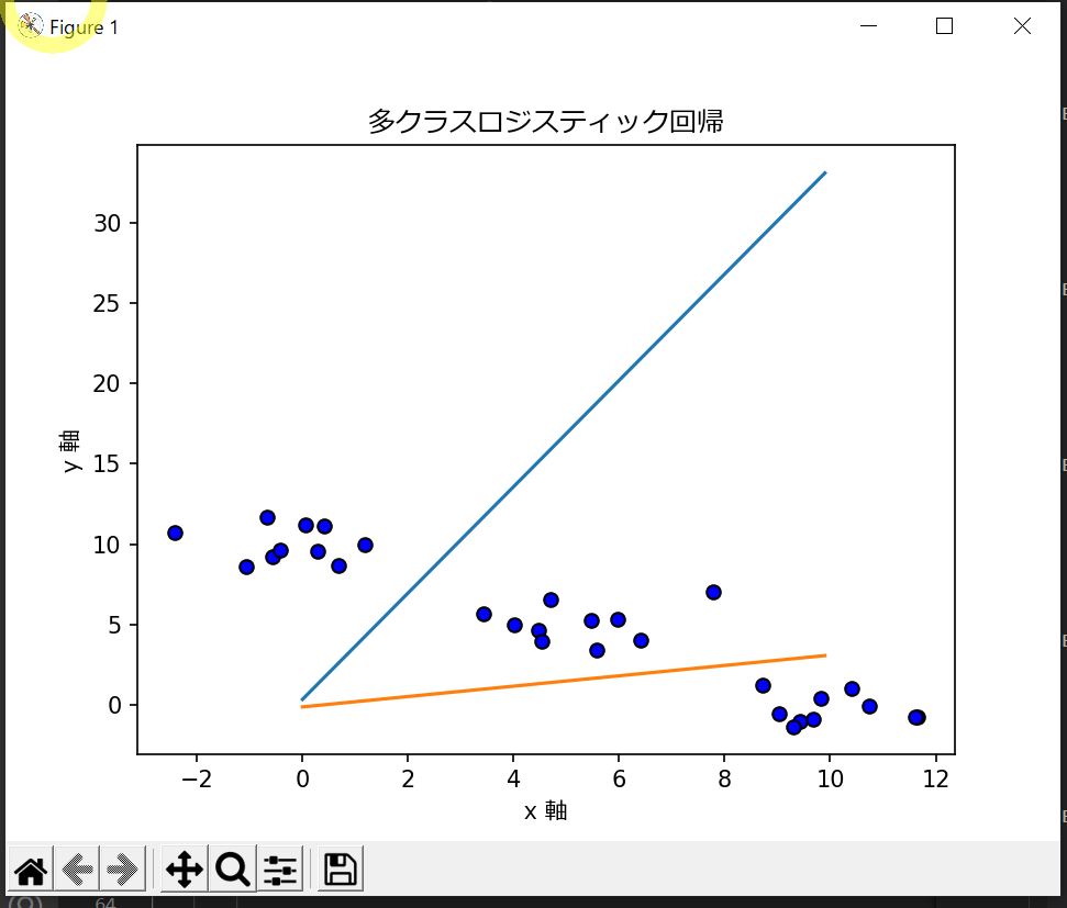
plt.title('多クラスロジスティック回帰',fontname="Meiryo")
# 描画関数
plt.show()
if __name__ == "__main__":
main()
(図131)
(例)出力結果
Epoc=  1 No. =  0
         x1,x2          = array([0.6383, 9.0615])
         t              = array([1., 0., 0.])
         w1,w2          = array([[0.,0.],[0.,0.],[0.,0.]])
         b              = array([[0.],[0.],[0.]])
         y              = array([[0.3333],[0.3333],[0.3333]])
         dw1,dw2        = array([[-1.471,-2.1043],[2.9419,4.2086],[-1.471,-2.1043]])
         db             = array([[-0.3333],[0.6667],[-0.3333]])
~中略~
Epoc=  30 No. =  29
         x1,x2          = array([10.632, -0.321])
         t              = array([0., 0., 1.])
         w1,w2          = array([[-1.9226,1.3133],[0.5322,0.5343],[1.3903,-1.8476]])
         b              = array([[-0.068],[0.14],[-0.072]])
         y              = array([[0.9891],[0.0109],[0.]])
         dw1,dw2        = array([[0.0159,0.1162],[-0.0159,-0.1162],[-0.,-0.]])
         db             = array([[0.0109],[-0.0109],[-0.]])