<目次>
オーバーフィッティング問題の具体例(Python-Keras)
概要
原因
(1-1) Pythonによる具体例
(1-2) 対策
(1-3) ニューラルネットワークの次数について
オーバーフィッティング問題の具体例(Python-Keras)
概要
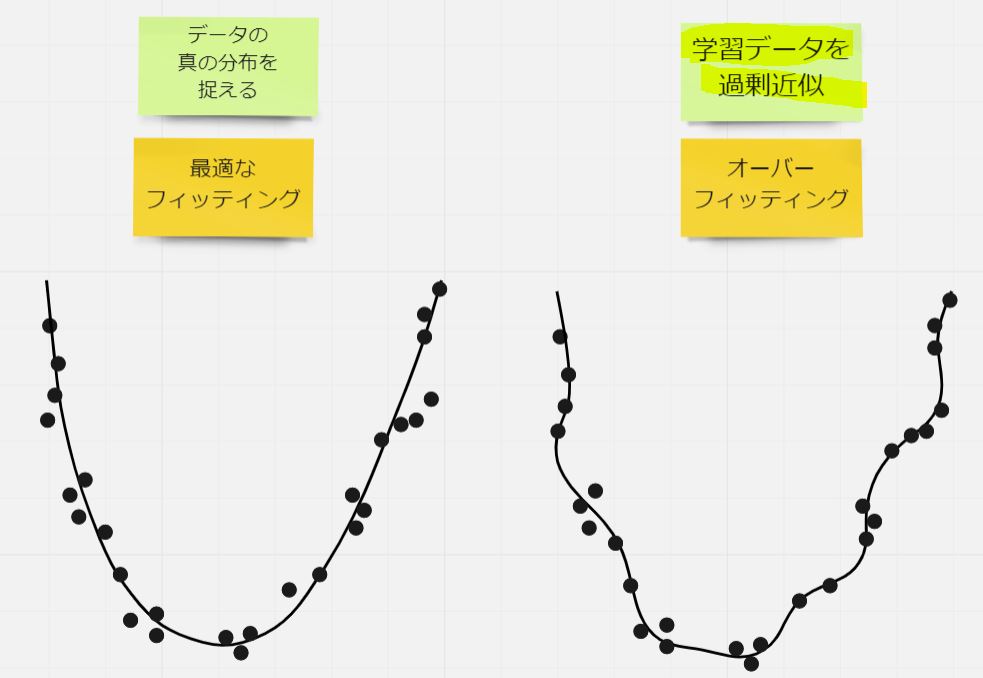
モデルの学習において、訓練データへの過剰な適合により、未知データへの汎化能力が低下する現象を「オーバーフィッティング」と呼びます。
特に高次元・高複雑なモデルでは、ノイズまで学習してしまい、結果として予測精度が下がることがあります。
(図110)
原因
オーバーフィッティングを引き起こす主な要因には以下があります:
- 活性化関数が高次すぎ、訓練データに過度に最適化された
- 隠れ層の数が多すぎる
- 隠れ層のニューロン数が多すぎる
これらはいずれも表現力の高いモデル構造である一方、訓練データへの過剰な適合を招き、未知データへの対応力を損なうリスクがあります。
そのため、誤差E(損失)を小さくしすぎることも必ずしも望ましくありません。
(1-1) Pythonによる具体例
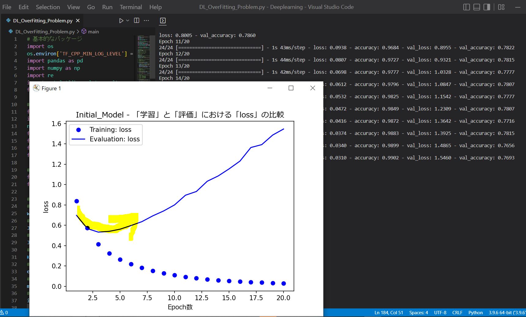
以下に、PythonとKerasを使ってオーバーフィッティングを再現したサンプルコードを掲載します。
学習が進むと loss の値が一定で頭打ちになり、学習がうまく進んでいない様子が確認できます。
# 基本的なパッケージ
import os
os.environ['TF_CPP_MIN_LOG_LEVEL'] = '3'
import pandas as pd
import numpy as np
import re
import matplotlib.pyplot as plt
from pathlib import Path

# データ準備のためのパッケージ
from sklearn.model_selection import train_test_split
import nltk as nltk
nltk.download("stopwords")
from nltk.corpus import stopwords
from keras.preprocessing.text import Tokenizer
from keras.utils.np_utils import to_categorical
from sklearn.preprocessing import LabelEncoder

# モデルを作るためのパッケージ
from keras.models import Sequential
from keras.layers import Dense, Activation

# 入力xの次元
# 突合用のdictionaryに保持する単語の数を指定
words_num = 10000
# 隠れ層haの次元(クラス数)
Ja = 64
# 隠れ層hbの次元(クラス数)
Jb = 64
# 出力yの次元(クラス数)
K = 3
# 学習のepoc数
epoch_num = 20
# ミニバッチ勾配降下法で利用するバッチサイズ
mini_batch_size = 512
# 入力データファイルのパス
input_path = Path('C:\\dev\\Python\\00_LocalPythonApp\\Deeplearning\\input\\')

# ■ 目的・用途
#  入力したPandas Seriesに対して、英語のstopwordsを除外する
# ■ 入力パラメータ
#  綺麗にしたいテキスト
# ■ 出力
#  stopwordsが除去されたPandas Series
def remove_stopwords(input_text):

    stopwords_list = stopwords.words('english')
    # 何かの感情を意味する可能性があるものは、whitelistに登録して削除の対象外にする
    whitelist = ["n't", "not", "no"]
    words = input_text.split()
    clean_words = [word for word in words if (word not in stopwords_list or word in whitelist) and len(word) > 1]
    return " ".join(clean_words)

# ■ 目的・用途
#  入力したPandas Seriesに対して、メンション(@XXXX)を削除する
# ■ 入力パラメータ
#  綺麗にしたいテキスト
# ■ 出力
#  メンションが除去されたPandas Series
def remove_mentions(input_text):

    return re.sub(r'@\w+', '', input_text)

# ■ 目的・用途
#  多クラスモデルの学習。epocやbatch_sizeはグローバル変数で指定。
# ■ 入力パラメータ
#  X_train : 学習の入力値
#   y_train : 学習の正解値
#   X_valid : 評価の入力値
#   Y_valid : 評価の正解値
# ■ 出力
#  モデルの学習履歴
def create_deeplearning_model(model, X_train, y_train, X_valid, y_valid):

    model.compile(loss='categorical_crossentropy', optimizer='rmsprop', metrics=['accuracy'])
    history = model.fit(X_train, y_train, epochs=epoch_num, batch_size=mini_batch_size, validation_data=(X_valid, y_valid))
    return history

def display_training_result(model,X_train,T_train,model_hist):

    # 分類が正しい結果になっているか?の確認
    # model.predict(X_train,batch_size=mini_batch_size)
    #  ⇒各「入力」に対する「出力」の確率(ソフトマックス)の確認
    # np.argmax(●)で[X,X,X]の最大のインデックスを抽出
    # (例) [[0,1,0],[0,0,1],[1,0,0]]⇒[1,2,0]
    # axis=1の場合は横軸単位で比較する。
    # axis=0の場合は縦軸同士で比較する。
    classes = np.argmax(model.predict(X_train,batch_size=mini_batch_size),axis=1)

    # 正解のインデックス情報
    #  t_でデータ数N回ループし、正解のindexを抽出してリスト化け
    #  (例)[[0,1,0],[0,0,1],[1,0,0]]⇒[1,2,0]
    t_index = np.argmax(T_train,axis=1)
    # 別の方法で、forループを使ったワンライナーでも記述可能。
    #t_index = [index for i in range(len(T_train)) for index in range(K) if T_train[i][index] == 1]

    # ネットワークの出力「y」の計算結果を取得
    prob = model.predict(X_train,batch_size=mini_batch_size)

    # 評価誤差が最小となるepoc番号
    min_epoch = np.argmin(model_hist.history['val_loss']) + 1

    print("*******************************")
    print("minimul loss epoch: {}".format(min_epoch))
    # 分類出来たか?はyの最大index(classes)と、tの最大index(T_trainindex)を比較
    print("classified: ",t_index==classes)
    print("probability: ",prob)
    print("*******************************")

# ■ 目的・用途
#  学習したモデルを、指定した指標(metric)で評価する。
#  学習と評価の内容はepoc単位でグラフに描画する。
# ■ 入力パラメータ
#  history:モデルの学習history
#  metric_name:loss / accuracy
# ■ 出力
#  x軸:epoc、y軸:指標の値
def eval_metric(model, history, metric_name):

    metric = history.history[metric_name]
    val_metric = history.history['val_' + metric_name]
    e = range(1, epoch_num + 1)
    plt.plot(e, metric, 'bo', label='Training: ' + metric_name)
    plt.plot(e, val_metric, 'b', label='Evaluation: ' + metric_name)
    plt.xlabel('Epoch数',fontname="Meiryo")
    plt.ylabel(metric_name)
    plt.title(model.name + ' - ' + '「学習」と「評価」における「'+ metric_name +'」の比較',fontname="Meiryo")
    plt.legend()
    plt.show()

def main():
    df = pd.read_csv(input_path / 'Tweets.csv')
    df = df.reindex(np.random.permutation(df.index))
    df = df[['text', 'airline_sentiment']]

    # 分析に不要な単語は除外する
    # (例)Twitterのメンション
    # (例)it's, you've, I, didn't, aなどのStemワード
    df.text = df.text.apply(remove_stopwords).apply(remove_mentions)

    # データを「学習用」と「テスト用」に分ける
    # X:Twitterの投稿文章
    # y:感情分析の正解(Positive/Negative/Neautral)
    X_train, X_test, T_train, T_test = train_test_split(df.text, df.airline_sentiment, test_size=0.1, random_state=37)

    # Xの方は文の状態なので、
    # Tokenizerで単語を分解してdictionaryに格納する
    # indexが小さい程、高頻度で登場する単語になる。
    tk = Tokenizer(num_words=words_num,
               filters='!"#$%&()*+,-./:;<=>?@[\\]^_`{"}~\t\n',
               lower=True,
               char_level=False,
               split=' ')
    tk.fit_on_texts(X_train)

    # 生成したdictionaryのindexと、各文章を突合したマトリクスを作成
    # (例)文章にindex=2の単語「am」がある ⇒ 2要素目に「1」を立てる
    #  ⇒[0. 1. 1. ... 0. 0. 0.]
    X_train_binary = tk.texts_to_matrix(X_train, mode='binary')
    X_test_binary = tk.texts_to_matrix(X_test, mode='binary')

    # y要素もLabelEncoderで値をラベル変換
    # 0:negative, 1:neutral, 2:positive
    # (例)[1 0 2 2 0 1 1 2]
    le = LabelEncoder()
    T_train_le = le.fit_transform(T_train)
    T_test_le = le.transform(T_test)

    # 0,1の2値に変換
    # (例)
    # [1 0 2 2]
    # ↓
    # [[0.1.0.][1.0.0.][0.0.1.][0.0.1.]]
    T_train_binary = to_categorical(T_train_le)
    T_test_binary = to_categorical(T_test_le)

    # トレーニング用と評価用(モデルパラメータをチューニング時に使用)に分解
    X_train_rest, X_valid, T_train_rest, T_valid = train_test_split(X_train_binary, T_train_binary, test_size=0.1, random_state=37)

    # モデルの生成
    init_model = Sequential()
    init_model.add(Dense(input_shape=(words_num,), units=Ja, activation='relu'))
    init_model.add(Dense(units=Jb, activation='relu'))
    init_model.add(Dense(units=K, activation='softmax'))
    init_model._name = 'Initial_Model'

    # モデルの学習
    init_history = create_deeplearning_model(init_model, X_train_rest, T_train_rest, X_valid, T_valid)

    # モデルの学習結果を表示
    display_training_result(init_model,X_train_rest,T_train_rest,init_history)

    # モデルの評価
    eval_metric(init_model, init_history, 'loss')

if __name__ == "__main__":
    main()
実行結果としては、Epoch=2〜3以降で誤差(loss)が頭打ちになり、学習が進まなくなる様子が観察できます。
(図141)
(1-2) 対策
※本節は別記事にてご紹介予定です。
(1-3) ニューラルネットワークの次数について
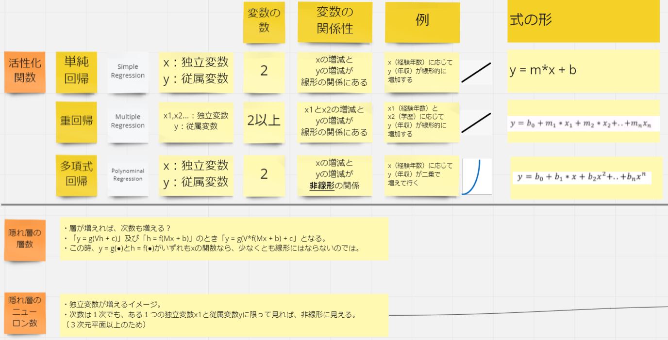
ニューラルネットワークの構造において、どこまでの「次数(複雑さ)」を持たせるかは非常に重要な設計要素です。
ただし本節の内容は一部裏付けが未完のため、参考程度にご覧ください。
(図151)