オーバーフィッティングの対策（ドロップアウト）をご紹介（Kerasプログラムあり）

＜目次＞

■オーバーフィッティングの対策（ドロップアウト）をご紹介（Kerasプログラムあり）
　■オーバーフィッティング問題とは？
　■対策の概要
　 ■(１-１) ドロップアウトの数式
　 ■(１-２) ドロップアウトの構文
　 ■(１-３) Kerasサンプルプログラム

■オーバーフィッティングの対策（ドロップアウト）をご紹介（Kerasプログラムあり）

■オーバーフィッティング問題とは？

オーバーフィッティングとは、学習データに対して過剰に適合してしまう問題です。これはモデルが学習データに含まれるノイズまでも覚えてしまい、汎化性能（未知データへの対応力）が低下する現象です。
→（参考）オーバーフィッティング問題とは？

＞目次にもどる

■対策の概要

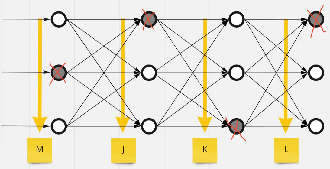
オーバーフィッティングへの代表的な対策として「ドロップアウト」があります。
これは、学習中にランダムに一定割合のニューロンを無効化（ドロップ）し、複数のネットワークを擬似的に構築するような手法です。
通常は確率P＝0.5などがよく用いられます。
予測・評価時にはドロップアウトを行わず、全体のネットワークで推論します。

（図121）

＞目次にもどる

■(１-１) ドロップアウトの数式

多層パーセプトロンに対するドロップアウトの数式は以下の通りです。
ベクトル \( \boldsymbol{m} \) をドロップアウト用マスクとし、多層パーセプトロンの基本アルゴリズムと比較します。

●正伝播（隠れ層→出力層の式）

\( \boldsymbol{h} = f(\boldsymbol{W} \boldsymbol{x} + \boldsymbol{b}) \)

↓

\( \boldsymbol{h} = f(\boldsymbol{W} \boldsymbol{x} + \boldsymbol{b}) \odot \boldsymbol{m} \)

●逆伝播（多層パーセプトロン）
\( \boldsymbol{W}^{(i+1)} \) \( \quad=\boldsymbol{W}^{(i)}+\eta f(\boldsymbol{p})(\boldsymbol{I}-f(\boldsymbol{p})) \odot \boldsymbol{V}^\mathsf{T} \begin{pmatrix} \frac{\partial E}{\partial q_{1}} \\ \vdots \\ \frac{\partial E}{\partial q_{k}} \\ \vdots \\ \frac{\partial E}{\partial q_{K}} \end{pmatrix} \boldsymbol{x}^\mathsf{T} \)
↓
\( \boldsymbol{W}^{(i+1)} \) \( \quad=\boldsymbol{W}^{(i)}+\eta f(\boldsymbol{p})(\boldsymbol{I}-f(\boldsymbol{p})) \odot \boldsymbol{m} \odot \boldsymbol{V}^\mathsf{T} \begin{pmatrix} \frac{\partial E}{\partial q_{1}} \\ \vdots \\ \frac{\partial E}{\partial q_{k}} \\ \vdots \\ \frac{\partial E}{\partial q_{K}} \end{pmatrix} \boldsymbol{x}^\mathsf{T} \)

＞目次にもどる

■(１-２) ドロップアウトの構文

以下にオーバーフィッティング問題が起きているKerasプログラムを掲載します。

→（参考）勾配消失問題とは？原因や対策についてもご紹介

以下にKerasでドロップアウトを適用する構文を示します。

from keras.layers.core import Dropout

# モデルの生成
init_model = Sequential()
init_model.add(Dense(units=Ja, activation='relu', input_shape=(words_num,)))
init_model.add(Dropout(0.5))  # Dropout追加
init_model.add(Dense(units=Jb, activation='relu'))
init_model.add(Dropout(0.5))  # Dropout追加
init_model.add(Dense(units=K, activation='softmax'))

＞目次にもどる

■(１-３) Kerasサンプルプログラム

以下にオーバーフィッティングが発生していたKerasプログラムに、ドロップアウト対応を施したコードを掲載します。

→（参考）勾配消失問題とは？

# 基本的なパッケージ
from mimetypes import init
import os
os.environ['TF_CPP_MIN_LOG_LEVEL'] = '3'
import pandas as pd 
import numpy as np
import re
import matplotlib.pyplot as plt
from pathlib import Path

# データ準備のためのパッケージ
from sklearn.model_selection import train_test_split
import nltk as nltk
nltk.download("stopwords")
from nltk.corpus import stopwords
from keras.preprocessing.text import Tokenizer
from keras.utils.np_utils import to_categorical
from sklearn.preprocessing import LabelEncoder

# モデルを作るためのパッケージ
from keras.models import Sequential
from keras.layers import Dense, Activation

# ★追記
# ドロップアウト対応用
from keras.layers.core import Dropout

# 入力xの次元
# 突合用のdictionaryに保持する単語の数を指定
words_num = 10000
# 隠れ層haの次元（クラス数）
Ja = 64
# 隠れ層hbの次元（クラス数）
Jb = 64
# 出力yの次元（クラス数）
K = 3
# 学習のepoc数
epoch_num = 20
# ミニバッチ勾配降下法で利用するバッチサイズ
mini_batch_size = 512
# 入力データファイルのパス
input_path = Path('C:\\dev\\Python\\00_LocalPythonApp\\Deeplearning\\input\\')

# ■ 目的・用途
# 　入力したPandas Seriesに対して、英語のstopwordsを除外する
# ■ 入力パラメータ
# 　綺麗にしたいテキスト
# ■ 出力
# 　stopwordsが除去されたPandas Series
def remove_stopwords(input_text):

    stopwords_list = stopwords.words('english')
    # 何かの感情を意味する可能性があるものは、whitelistに登録して削除の対象外にする
    whitelist = ["n't", "not", "no"]
    words = input_text.split() 
    clean_words = [word for word in words if (word not in stopwords_list or word in whitelist) and len(word) > 1] 
    return " ".join(clean_words) 

# ■ 目的・用途
# 　入力したPandas Seriesに対して、メンション（@XXXX）を削除する
# ■ 入力パラメータ
# 　綺麗にしたいテキスト
# ■ 出力
# 　メンションが除去されたPandas Series  
def remove_mentions(input_text):

    return re.sub(r'@\w+', '', input_text)

# ■ 目的・用途
# 　多クラスモデルの学習。epocやbatch_sizeはグローバル変数で指定。
# ■ 入力パラメータ
# 　X_train : 学習の入力値
#   y_train : 学習の正解値
#   X_valid : 評価の入力値
#   Y_valid : 評価の正解値
# ■ 出力
# 　モデルの学習履歴 
def create_deeplearning_model(model, X_train, y_train, X_valid, y_valid):

    model.compile(loss='categorical_crossentropy', optimizer='rmsprop', metrics=['accuracy'])
    history = model.fit(X_train, y_train, epochs=epoch_num, batch_size=mini_batch_size, validation_data=(X_valid, y_valid))
    return history

def display_training_result(model,X_train,T_train,model_hist):

    # 分類が正しい結果になっているか？の確認
    # model.predict(X_train,batch_size=mini_batch_size)
    # 　⇒各「入力」に対する「出力」の確率（ソフトマックス）の確認
    # np.argmax(●)で[X,X,X]の最大のインデックスを抽出
    # (例) [[0,1,0],[0,0,1],[1,0,0]]⇒[1,2,0]
    # axis=1の場合は横軸単位で比較する。
    # axis=0の場合は縦軸同士で比較する。
    classes = np.argmax(model.predict(X_train,batch_size=mini_batch_size),axis=1)
    
    # 正解のインデックス情報
    # 　t_でデータ数N回ループし、正解のindexを抽出してリスト化け
    #　 (例)[[0,1,0],[0,0,1],[1,0,0]]⇒[1,2,0]
    t_index = np.argmax(T_train,axis=1)    
    # 別の方法で、forループを使ったワンライナーでも記述可能。
    #t_index = [index for i in range(len(T_train)) for index in range(K) if T_train[i][index] == 1]
    
    # ネットワークの出力「y」の計算結果を取得
    prob = model.predict(X_train,batch_size=mini_batch_size)

    # 評価誤差が最小となるepoc番号 
    min_epoch = np.argmin(model_hist.history['val_loss']) + 1

    print("*******************************")
    print("minimul loss epoch: {}".format(min_epoch))
    # 分類出来たか？はyの最大index(classes)と、tの最大index(T_trainindex)を比較
    print("classified: ",t_index==classes)
    print("probability: ",prob)
    print("*******************************")

# ■ 目的・用途
# 　学習したモデルを、指定した指標（metric）で評価する。
# 　学習と評価の内容はepoc単位でグラフに描画する。
# ■ 入力パラメータ
# 　history：モデルの学習history
# 　metric_name：loss / accuracy
# ■ 出力
# 　x軸:epoc、y軸:指標の値
def eval_metric(model, history, metric_name):

    metric = history.history[metric_name]
    val_metric = history.history['val_' + metric_name]
    e = range(1, epoch_num + 1)
    plt.plot(e, metric, 'bo', label='Training: ' + metric_name)
    plt.plot(e, val_metric, 'b', label='Evaluation: ' + metric_name)
    plt.xlabel('Epoch数',fontname="Meiryo")
    plt.ylabel(metric_name)
    plt.title(model.name + ' - ' + '「学習」と「評価」における「'+ metric_name +'」の比較',fontname="Meiryo")
    plt.legend()
    plt.show()

def main():
    df = pd.read_csv(input_path / 'Tweets.csv')
    df = df.reindex(np.random.permutation(df.index))  
    df = df[['text', 'airline_sentiment']]
    
    # 分析に不要な単語は除外する
    # （例）Twitterのメンション
    # （例）it's, you've, I, didn't, aなどのStemワード
    df.text = df.text.apply(remove_stopwords).apply(remove_mentions)

    # データを「学習用」と「テスト用」に分ける
    # X：Twitterの投稿文章
    # y：感情分析の正解（Positive/Negative/Neautral）
    X_train, X_test, T_train, T_test = train_test_split(df.text, df.airline_sentiment, test_size=0.1, random_state=37)

    # Xの方は文の状態なので、
    # Tokenizerで単語を分解してdictionaryに格納する
    # indexが小さい程、高頻度で登場する単語になる。
    tk = Tokenizer(num_words=words_num,
               filters='!"#$%&()*+,-./:;<=>?@[\\]^_`{"}~\t\n',
               lower=True,
               char_level=False,
               split=' ')
    tk.fit_on_texts(X_train)

    # 生成したdictionaryのindexと、各文章を突合したマトリクスを作成
    # （例）文章にindex=2の単語「am」がある　⇒ 2要素目に「1」を立てる
    # 　⇒[0. 1. 1. ... 0. 0. 0.]
    X_train_binary = tk.texts_to_matrix(X_train, mode='binary')
    X_test_binary = tk.texts_to_matrix(X_test, mode='binary')

    # y要素もLabelEncoderで値をラベル変換
    # 0:negative, 1:neutral, 2:positive
    # （例）[1 0 2 2 0 1 1 2]
    le = LabelEncoder()
    T_train_le = le.fit_transform(T_train)
    T_test_le = le.transform(T_test)

    # 0,1の2値に変換
    # （例）
    # [1 0 2 2]
    # ↓
    # [[0.1.0.][1.0.0.][0.0.1.][0.0.1.]]
    T_train_binary = to_categorical(T_train_le)
    T_test_binary = to_categorical(T_test_le)

    # トレーニング用と評価用（モデルパラメータをチューニング時に使用）に分解
    X_train_rest, X_valid, T_train_rest, T_valid = train_test_split(X_train_binary, T_train_binary, test_size=0.1, random_state=37)

    # モデルの生成
    init_model = Sequential()
    init_model.add(Dense(units=Ja, activation='relu', input_shape=(words_num,)))
    # ★追記
    init_model.add(Dropout(0.5))
    init_model.add(Dense(units=Jb, activation='relu'))
    # ★追記
    init_model.add(Dropout(0.5))
    init_model.add(Dense(units=K, activation='softmax'))
    init_model._name = 'Initial_Model'

    # モデルの学習
    init_history = create_deeplearning_model(init_model, X_train_rest, T_train_rest, X_valid, T_valid)

    # モデルの学習結果を表示
    display_training_result(init_model,X_train_rest,T_train_rest,init_history)

    # モデルの評価
    eval_metric(init_model, init_history, 'loss')

if __name__ == "__main__":
    main()

（図131）Before

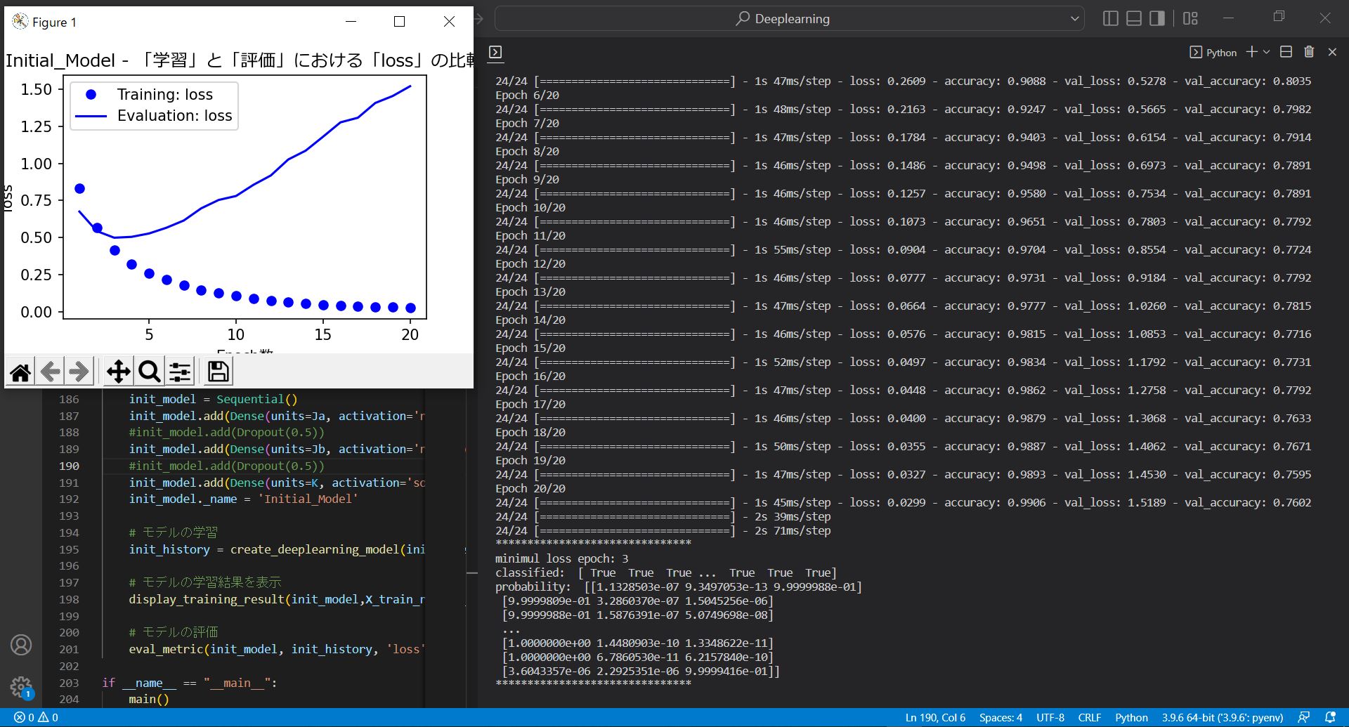
Epoch 19/20
24/24 [==============================] - 1s 47ms/step - loss: 0.0327 - accuracy: 0.9893 - val_loss: 1.4530 - val_accuracy: 0.7595
Epoch 20/20
24/24 [==============================] - 1s 45ms/step - loss: 0.0299 - accuracy: 0.9906 - val_loss: 1.5189 - val_accuracy: 0.7602

（図132）After

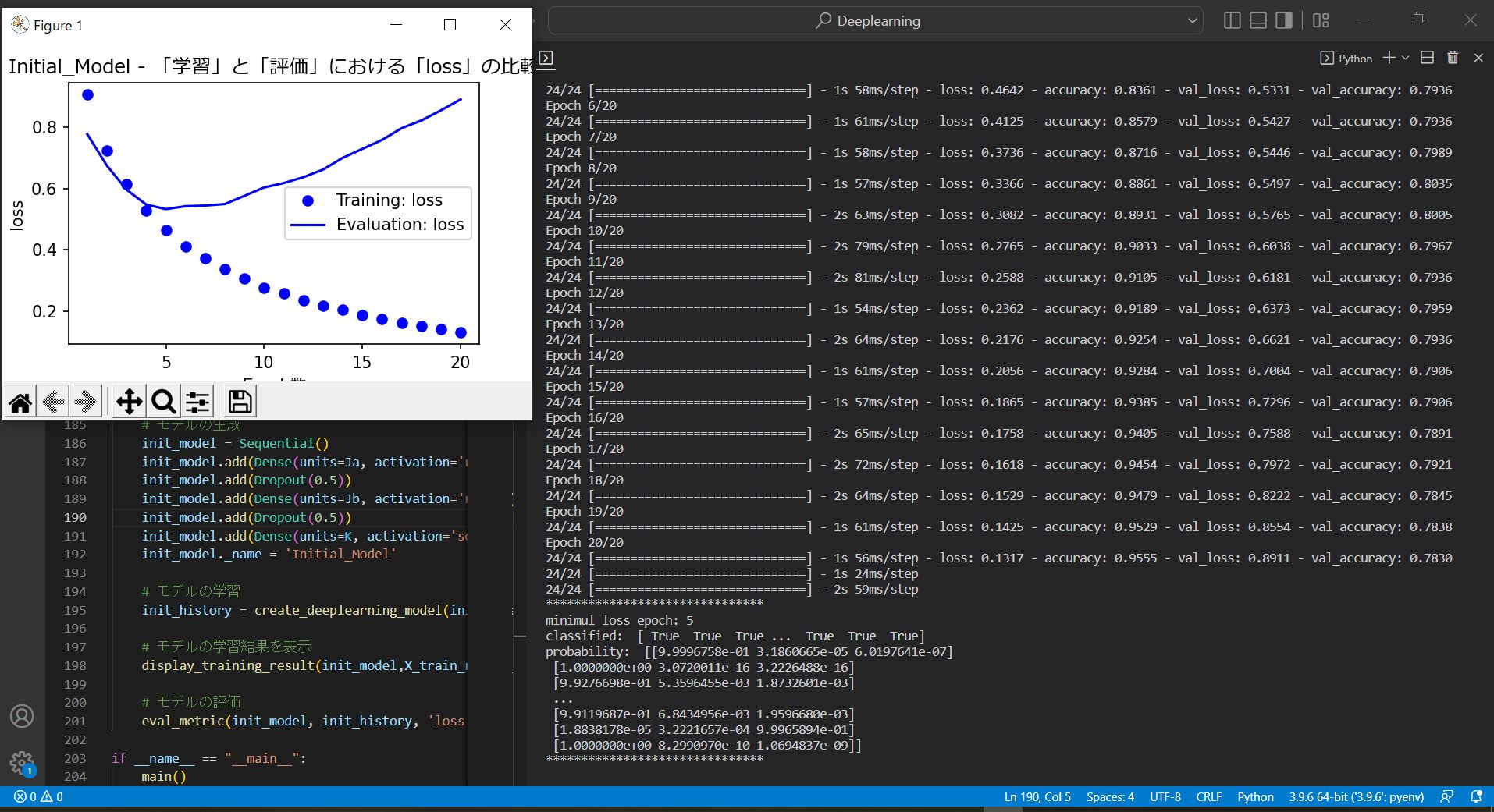
Epoch 19/20
24/24 [==============================] - 1s 61ms/step - loss: 0.1425 - accuracy: 0.9529 - val_loss: 0.8554 - val_accuracy: 0.7838      
Epoch 20/20
24/24 [==============================] - 1s 56ms/step - loss: 0.1317 - accuracy: 0.9555 - val_loss: 0.8911 - val_accuracy: 0.7830

このように、ドロップアウトを導入することで、学習精度を保ちつつ評価精度が改善される傾向が見られます。

＞目次にもどる